Closest Eredivisie football club

library(tidyverse)
library(sf)

Eredivisie clubs

The Eredivisie website has a page listing the 18 clubs currently in the league. Every club has its own page (for example, Ajax) which lists various statistics about the club, the players, and the stadium. Using rvest and jsonlite, we collect this list of clubs, and for every club obtain the stadium’s address. As a bonus, we collect the clubs’ logos, which will allow for nice plotting.

library(rvest)

url <- "https://eredivisie.nl/en-us/clubs"

club_names <- read_html(url) %>% 
  html_nodes(".clubs-list__club img") %>% 
  html_attr("title")


get_address <- function(club) {
  club <- URLencode(club)
  url <- "https://eredivisie.nl/en-us/API/DotControl/DCEredivisieLive/Stats/GetThemeSelection?teamname={club}&cid=0&moduleId=1261&tabId=255"

  str_glue(url) %>% 
    jsonlite::read_json() %>% 
    purrr::pluck("club", "stadium")
}

img_src <- "https://eredivisie-images.s3.amazonaws.com/Eredivisie%20images/Eredivisie%20Badges/{teamId}/150x150.png"

stadiums <- map_dfr(club_names, get_address) %>% 
  mutate(img = str_glue(img_src))

stadiums %>% 
  transmute(teamname, adres, city,
            img = cell_spec(stringr::str_trunc(img, 40, side = "left"),
                            "html", link = img)) %>% 
  head() %>% 
  knitr::kable(escape = FALSE) %>% 
  kable_styling(bootstrap_options = c("condensed", "hover"), font_size = 13) 

teamname	adres	city	img
Ajax	ArenA Boulevard 29	Amsterdam	…s/Eredivisie%20Badges/215/150x150.png
PSV	Frederiklaan 8	Eindhoven	…s/Eredivisie%20Badges/204/150x150.png
AZ	Stadionweg 1	Alkmaar	…s/Eredivisie%20Badges/313/150x150.png
Vitesse	Batavierenweg 25	Arnhem	…s/Eredivisie%20Badges/232/150x150.png
Feyenoord	Van Zandvlietplein 1	Rotterdam	…s/Eredivisie%20Badges/198/150x150.png
FC Groningen	Boumaboulevard 41	Groningen	…s/Eredivisie%20Badges/425/150x150.png

The addresses do not yet allow for plotting on a map — for that, we need coordinates. Converting a human-readable address into coordinates (such as latitude and longitude) is called geocoding. There are various APIs that do this. Most of these are paid, but I’ve found a free one that does the job. We provide it with an address as a string, and it gives us back the latitude and longitude. We have to be as specific as possible, to prevent it from finding a location with the same address in another country for example.

geo_locate <- function(address) {
  query_string <- URLencode(address)
  url <- "https://api.opencagedata.com/geocode/v1/json?q={query_string}&key=e5580345eb0e46d9a2e17e6a7e2373f7&no_annotations=1&language=nl"

  str_glue(url) %>% 
    jsonlite::read_json() %>% 
    purrr::pluck("results", 1, "geometry")
}

stadiums <- stadiums %>% 
  mutate(latlon = map(str_glue("{adres}, {postalcode} {city}, Nederland"), geo_locate)) %>% 
  unnest_wider(latlon)

stadiums %>% 
  transmute(teamname, lat, lng,
            img = cell_spec(stringr::str_trunc(img, 40, side = "left"),
                            "html", link = img)) %>% 
  head() %>% 
  knitr::kable(escape = FALSE) %>% 
  kable_styling(bootstrap_options = c("condensed", "hover"), font_size = 13) 

teamname	lat	lng	img
Ajax	52.31435	4.942843	…s/Eredivisie%20Badges/215/150x150.png
PSV	51.44083	5.477780	…s/Eredivisie%20Badges/204/150x150.png
AZ	52.61295	4.740751	…s/Eredivisie%20Badges/313/150x150.png
Vitesse	51.96366	5.893330	…s/Eredivisie%20Badges/232/150x150.png
Feyenoord	51.89434	4.524698	…s/Eredivisie%20Badges/198/150x150.png
FC Groningen	53.20702	6.591678	…s/Eredivisie%20Badges/425/150x150.png

Now that we have the clubs’ locations, we can do some data wrangling in order to create the map.

Map of the Netherlands

In order to plot a map of the Netherlands, we need the geometry of its boundaries. Below, we obtain municipality boundaries from the CBS (the Dutch national statistics bureau). From this, the country boundaries can be obtained with sf::st_union(). Since the CBS data is in a Dutch coordinate system called Rijksdriehoekscoördinaten, we first convert this to WGS84 via st_transform().

municipalities <- st_read("https://geodata.nationaalgeoregister.nl/cbsgebiedsindelingen/wfs?request=GetFeature&service=WFS&version=2.0.0&typeName=cbs_gemeente_2021_gegeneraliseerd&outputFormat=json", quiet = TRUE) %>% 
  st_transform(4326) # WGS84

nl <- st_union(municipalities)

ggplot(municipalities) +
  geom_sf() +
  theme_void()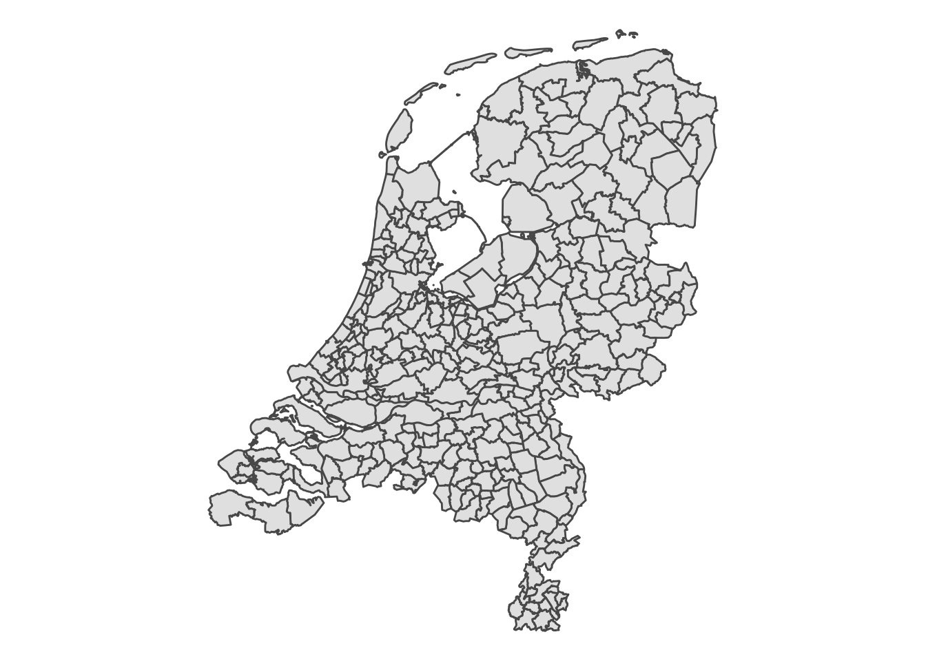

Voronoi

The type of map we want to generate is called a Voronoi diagram. We can create a Voronoi diagram from a set of points using sf::st_voronoi(). Since that function operates on a multipoint and we want the result to be of type sf, we do some pre- and post-processing.

voronoi <- stadiums %>% 
  select(lng, lat) %>% 
  as.matrix() %>% 
  st_multipoint() %>%
  st_voronoi(envelope = nl) %>%
  st_collection_extract() %>% 
  st_set_crs(4326) %>% # WGS84
  st_sf()

plot(voronoi)
stadiums %>% 
  select(lng, lat) %>% 
  as.matrix() %>% 
  points()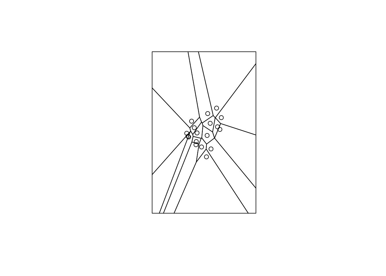

Now that we have the Voronoi diagram, we can join it to the stadium data. We intersect it with the boundaries of the Netherlands to make sure the Voronoi lines do not extend to outside the country borders.

stadiums_voronoi <- stadiums %>%
  st_as_sf(coords = c("lng", "lat"),
           crs = 4326, remove = FALSE) %>% 
  st_join(voronoi, .) %>% # join makes sure we map each tile to the correct centroid
  st_cast("MULTILINESTRING") %>% # turn polygons into lines
  st_intersection(nl) # within NL

Plotting

Finally, we can plot the map of the Netherlands together with the club logos and the Voronoi edges.
We do some manual work to move the club logos away from the points, to make the plot look nicer. The result is a map of the closest Eredivisie football club!

offsets <- tribble(~ teamname, ~ dlng, ~dlat,
                   "Feyenoord", 0.12, -0.12,
                   "Sparta Rotterdam", -0.15, -0.13,
                   "Fortuna Sittard", -0.15, -0.1,
                   "PSV", 0.12, 0.1,
                   "Willem II", 0, -0.15,
                   "RKC Waalwijk", 0.13, 0.08,
                   "ADO Den Haag", 0.1, 0.1,
                   "Ajax", 0.05, 0.14,
                   "FC Utrecht", 0.1, 0.08,
                   "AZ", 0.08, 0.1,
                   "Vitesse", 0.05, -0.15,
                   "FC Twente", 0.12, 0.1,
                   "Heracles Almelo", -0.1, -0.15,
                   "PEC Zwolle", 0, -0.14,
                   "sc Heerenveen", -0.1, 0.15,
                   "FC Groningen", -0.15, -0.1,
                   "FC Emmen", 0.14, 0.1,
                   "VVV-Venlo", -0.1, 0.1)

stadiums_voronoi %>% 
  left_join(offsets, by = "teamname") %>% 
  mutate(lng_img = lng + dlng,
         lat_img = lat + dlat) %>% 
  ggplot() +
  geom_sf(data = municipalities, size = 0.1, fill = "#cccccc") +
  geom_sf(size = 0.6, fill = NA, color = "black", alpha = 0.8) +
  ggimage::geom_image(aes(image = img, x = lng_img, y = lat_img), size = 0.08) + 
  geom_point(aes(x = lng, y = lat)) +
  theme_void()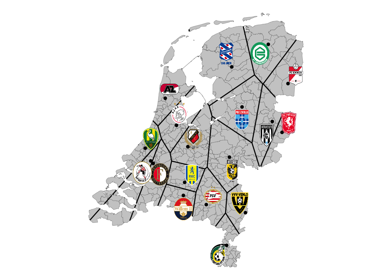

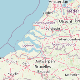
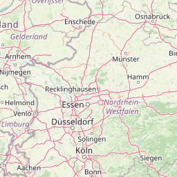
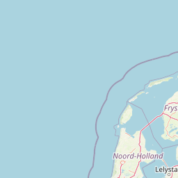
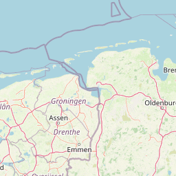
Bonus: interactive map

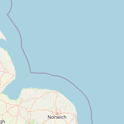
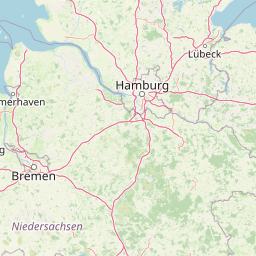
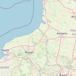
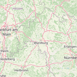
Using the leaflet library, it is easy to create an interactive map in R. Below, we show the Netherlands with OpenStreetMap, and draw the Voronoi boundaries and markers for the stadiums on top of it. Adding images to leaflet is not straightforward, so we will not add these.

library(leaflet)

stadiums %>%
  st_as_sf(coords = c("lng", "lat"),
           crs = 4326, remove = FALSE) %>% 
  st_join(voronoi, .) %>% # join makes sure we map each tile to the correct centroid
  st_cast("MULTILINESTRING") %>% # turn polygons into lines
  leaflet() %>% 
  setView(lng = 5.6, lat = 52.2, zoom = 7) %>%
  addTiles() %>% 
  addMarkers(lng = ~lng, lat = ~lat, label = ~teamname) %>% 
  addPolylines()