Riddler: Can You Eat All The Chocolates?

Simulation in R

The following R function simulates eating one bag of chocolates and outputs what the last chocolate was.

chocolates <- c(rep("m", 2), rep("d", 8))

eat_chocolates <- function() {
  # shuffle the chocolates around
  chocolates_left <- sample(chocolates)
  
  # eat the first chocolate
  last_taken <- chocolates_left[1]
  chocolates_left <- chocolates_left[-1]
  
  # eat the rest of the chocolates
  while (length(chocolates_left) > 0) {
    # take the first chocolate out of the bag
    to_eat <- chocolates_left[1]
    chocolates_left <- chocolates_left[-1]
    
    # put back and shuffle if differs from previous piece
    if (to_eat != last_taken) {
      chocolates_left <- sample(c(to_eat, chocolates_left))
    }
    
    last_taken <- to_eat
  }
  
  last_taken
}

We can now easily run, for example, 100,000 simulations and calculate the percentage in which the last chocolate was milk:

simulations <- replicate(1e5, eat_chocolates())
mean(simulations == "m")

## [1] 0.46348

In a couple of seconds, this gives an estimate of a 46% probability of ending with a piece of milk chocolate. This is closer to 50% than I initially expected. Intuitively though, it does make sense, given the nature of the problem that the majority chocolate type will be eaten relatively quickly, since it is easier to get a ‘streak’ of those.

Running this (admittedly naive) simulation for more than, say, 1 million replications quickly becomes intractable. For a more accurate result that does run quickly, we can resort to recursion.

Recursion

The problem ca be written in a recursive form: given a number of milk and dark chocolates, we can create a set of possible next states and attach probabilities to those states. We can repeat this until we arrive at a bag of only one type of chocolate.

In order to do that, let’s first introduce some notation. Let \(P(m, d, x)\) be the probability of ending with a milk chocolate given that we currently have a bag of \(m\) milk and \(d\) dark chocolates and that the last chocolate we ate was of type \(x\in\{\text{milk}, \text{dark}\}\). Denote by \(x^c\) the chocolate type that is not \(x\). We then know the trivial cases \(P(m, 0, x) = 1\) and \(P(0,d,x)=0\); you can’t “fail” if you only have milk left, and you can’t “succeed” if you only have dark chocolates left.

Moreover, the probability of ending with a milk chocolate given a certain distribution of chocolates and a previous pick equals the probability of ending with a dark chocolate given that we have switched all dark and milk chocolates around. In mathematical terms, \(P(m,d|x) = 1-P(d,m|x^c)\).

Now, given a state \((m,d, \text{milk})\), you will pick a milk chocolate with probability \(\frac{m}{m+d}\), resulting in a state of \((m-1, d, \text{milk})\), or you will pick dark with probability \(\frac{d}{m+d}\), resulting in \((m, d, \text{dark})\). In other words, given \(m,d>0\),\[ P(m, d, \text{milk}) = \frac{m}{m+d}\cdot P(m-1,d,\text{milk})\,+\,\frac{d}{m+d}\cdot P(m,d,\text{dark}). \]

We can now immediately see a problem with programming this recursion as it is: the second term did not decrease the total number of chocolates. Were we to do another step, we could again arrive at the situation we started with, thus resulting in an endless loop. In other words, theoretically we could keep alternately picking \(\text{milk}\) and \(\text{dark}\) chocolates and never finish the whole bag.

We need to go deeper.

Let’s do another recursion step by expanding the right-most term in the above equation:

\[ P(m,d,\text{dark}) = \frac{m}{m+d}\cdot P(m,d,\text{milk})\,+\,\frac{d}{m+d}\cdot P(m,d-1,\text{dark}). \]

Filling this into the first equation,

\[ P(m, d, \text{milk}) = \frac{m}{m+d}\cdot P(m-1,d,\text{milk})\,+\,\frac{d}{m+d}\cdot \left(\frac{m}{m+d}\cdot P(m,d,\text{milk})\,+\,\frac{d}{m+d}\cdot P(m,d-1,\text{dark})\right), \]

which we can rearrange into

\[ P(m, d, \text{milk}) - \frac{md}{(m+d)^2}\cdot P(m,d,\text{milk}) = \frac{m}{m+d}\cdot P(m-1,d,\text{milk})\,+\,\frac{d^2}{(m+d)^2}\cdot P(m,d-1,\text{dark}), \]

or

\[ \frac{(m+d)^2-md}{(m+d)^2}\cdot P(m,d,\text{milk}) = \frac{m}{m+d}\cdot P(m-1,d,\text{milk})\,+\,\frac{d^2}{(m+d)^2}\cdot P(m,d-1,\text{dark}), \]

which gives

\[ P(m,d,\text{milk}) = \frac{m^2+md}{m^2+d^2+md}\cdot P(m-1,d,\text{milk})\,+\,\frac{d^2}{m^2+d^2+md}\cdot P(m,d-1,\text{dark}). \]

Now, by magic, this recursion does strictly decrease the total number of chocolates in the bag, thus making a program feasible. Together with the relationship \(P(m,d,\text{dark})=1-P(d,m,\text{milk})\), we can calculate our quantity of interest, which is the probability of ending with a milk chocolate given a starting bag and no previous chocolates eaten:

\[ P(m,d)=\frac{m}{m+d}\cdot P(m-1,d,\text{milk})\,+\,\frac{d}{m+d}\cdot P(m,d-1,\text{dark}). \]

In R code, this recursion can be programmed as follows.

P <- function(m, d, previous = "") {
  if (m == 0) {
    return(0)
  } else if (d == 0) {
    return(1)
  }
  
  if (previous == "") {
    m/(m+d)*P(m-1, d, "milk") + d/(m+d)*P(m, d-1, "dark")
  } else if (previous == "milk") {
    (m^2+m*d)/(m^2+d^2+m*d)*P(m-1, d, "milk") + (d^2)/(m^2+d^2+m*d)*P(m, d-1, "dark")
  } else if (previous == "dark") {
    1 - P(d, m, "milk")
  }
}

This allows us to calculate some simple examples,

P(2,0)

## [1] 1

P(0,2)

## [1] 0

P(1,1)

## [1] 0.5

but also the actual quantity of interest

P(2,8)

## [1] 0.4615372

within a second. This agrees with the outcome of our simulation: the probability of ending with a milk chocolate is about 46.15%.

Other starting points

Now that we have code that runs quickly, we can explore the probabilities for other mixes of chocolates.

Say we start with 2 milk chocolates, but vary the number of dark chocolates.

library(tidyverse)
theme_set(theme_light())

simulations <- tibble(m = 2, d = 1:100) %>% 
  rowwise() %>% 
  mutate(p = P(m, d))

ggplot(simulations, aes(d, p)) + 
  geom_line() +
  scale_y_continuous(labels = scales::percent_format()) +
  labs(title = "Probability of ending with a milk chocolate",
       subtitle = "Given 2 milk and a varying number of dark chocolates",
       x = "Number of dark chocolates",
       y = "Probability")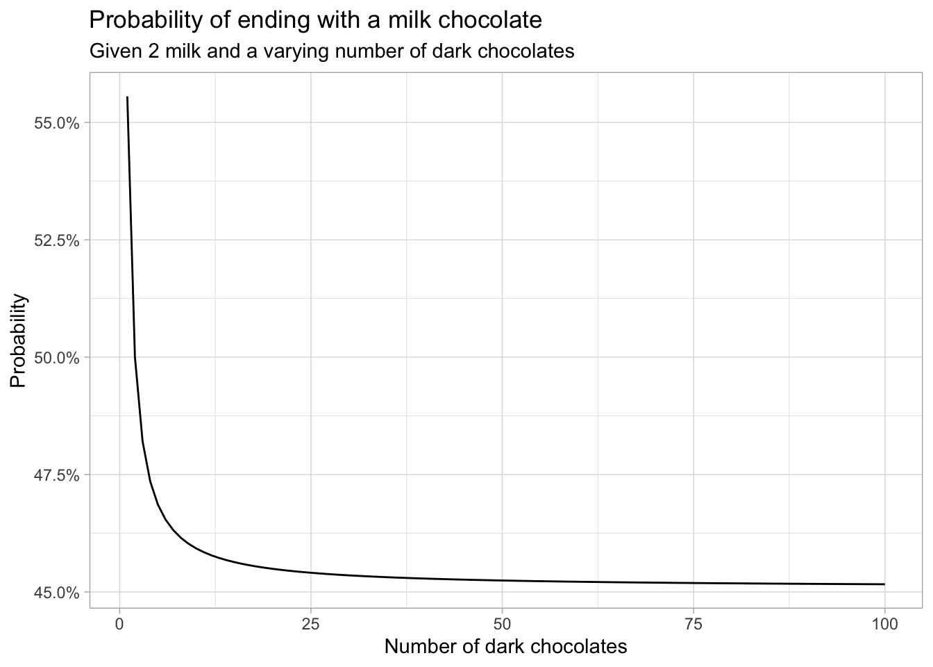

At first, the probability of success drops quickly, but at some point the streaks of dark chocolates will be so common that adding more dark chocolates does not decrease this probability significantly.

We can do the same thing in two dimensions by also varying the number of milk chocolates. Now, memoization comes in handy, since otherwise we calculate the same probability many times. The function P_mem calculates P but checks whether a certain probability has already been calculated in the list of matrices mem.

n_max <- 20
mem <- list(milk = matrix(nrow = n_max, ncol = n_max),
            dark = matrix(nrow = n_max, ncol = n_max))

P_mem <- function(m, d, previous = "") {
  if (m == 0) {
    return(0)
  } else if (d == 0) {
    return(1)
  }
  
  if (previous != "" && !is.na(mem[[previous]][m, d])) {
    return(mem[[previous]][m, d])
  }
  
  if (previous == "") {
    res <- m/(m+d)*P_mem(m-1, d, "milk") + d/(m+d)*P_mem(m, d-1, "dark")
  } else if (previous == "milk") {
    res <- (m^2+m*d)/(m^2+d^2+m*d)*P_mem(m-1, d, "milk") + (d^2)/(m^2+d^2+m*d)*P_mem(m, d-1, "dark")
    mem[[previous]][m, d] <<- res
  } else if (previous == "dark") {
    res <- 1 - P_mem(d, m, "milk")
    mem[[previous]][m, d] <<- res
  }
  
  res
}

simulations <- crossing(m = 1:n_max, d = 1:n_max) %>% 
  rowwise() %>% 
  mutate(p = P_mem(m, d))

ggplot(simulations, aes(m, d, fill = p)) + 
  geom_raster() +
  scale_fill_continuous(labels = scales::percent_format()) +
  labs(title = "Probability of ending with a milk chocolate",
       x = "Number of milk chocolates",
       y = "Number of dark chocolates",
       fill = "Probability")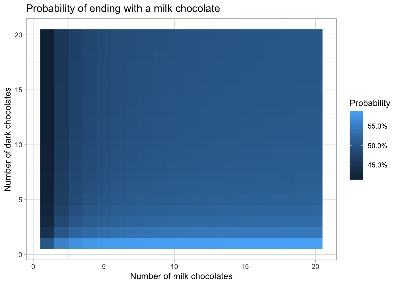

This graph shows that the more chocolates there are in the bag, the smaller the differences between different mixes become.