An image can be viewed as a function mapping pixel locations \(x,y\) to color values \(R,G,B\). Since neural networks are function approximators, we can train such a network to approximate an image. The network is then a representation of the image as a function and its contents can be displayed by evaluating the network for all pixel pairs \(x,y\).

The Keras package for R is now approximately 1 year old but I have to admit that I usually go to Python to implement neural networks. Since I wanted to try the imager package for R for a while, let’s hit two birds with one stone and do this exercise in R.

First, we need the right packages.

library(tidyverse)
library(keras)
library(imager)

To honour the name of this blog, let’s pick an image of the bird species godwit (scientific name: limosa) and load it using imager’s load.image.

# Image from Pixabay
im_url <- "https://cdn.pixabay.com/photo/2015/09/18/00/13/bar-tailed-godwit-944883_640.jpg"
im <- load.image(im_url)
dim(im)

## [1] 640 480   1   3

The image is 640x480 pixels in size, consists of 1 frame (it is not a video) and 3 color channels.
Plotting the image is easy. We choose to show the image without axes and make the margins small for aestetic reasons.

plot(im, axes = FALSE)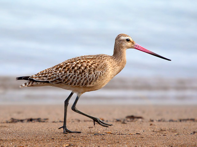

A godwit. Source: pixabay.com

We convert the image to a data frame by calling as.data.frame on the image object. This data frame by default has 4 columns: an x and y column to identify each pixel’s location, a color channel column cc, and the value this channel takes at this pixel. We spread the key-value pairs in the cc and value columns into columns cc_1, cc_2, cc_3 representing the three color values.

df <- im %>% as.data.frame %>% spread(cc, value)
head(df)

##   x y         1         2         3
## 1 1 1 0.8117647 0.8941176 0.9607843
## 2 1 2 0.8117647 0.8941176 0.9607843
## 3 1 3 0.8117647 0.8941176 0.9607843
## 4 1 4 0.8117647 0.8980392 0.9529412
## 5 1 5 0.8196078 0.8941176 0.9529412
## 6 1 6 0.8117647 0.8862745 0.9450980

The color values are between 0 (absent) and 1 (present).
We create input and output matrices which can be fed into keras.

X <- as.matrix(select(df, x, y))
Y <- as.matrix(select(df, -x, -y))

Creating a neural network with keras is very easy. We tell it that we want an ‘ordinary’ feed forward neural network with keras_model_sequential(). For starters, we create a one-layer network with 2 input nodes (x and y coordinates) and 3 output nodes (R, G, B values). We choose a ‘sigmoid’ activation function because we want the output values to be between 0 and 1.

model <- keras_model_sequential() 
model %>%
  layer_dense(3, input_shape = 2, activation = "sigmoid")
summary(model)

## ___________________________________________________________________________
## Layer (type)                     Output Shape                  Param #     
## ===========================================================================
## dense_1 (Dense)                  (None, 3)                     9           
## ===========================================================================
## Total params: 9
## Trainable params: 9
## Non-trainable params: 0
## ___________________________________________________________________________

When compiling the model, we tell it what loss function we need, what optimizer and what kind of metrics we want it to display while training. We choose a mean_squared_error loss, which means that we penalize every color channel equally, taking the square of the error for every channel and every pixel. We optimize the network using the widely used Adam optimizer and we want to see its accuracy while training.

model %>% compile(
  loss = "mean_squared_error",
  optimizer = optimizer_adam(),
  metrics = "accuracy"
)

Next, we actually fit the model, giving it the expected input and output matrices X and Y. We set the batch size to 128 such that training is faster than the default 32. We train the network for 20 epochs.

model %>% fit(
  X, Y, 
  batch_size = 128,
  epochs = 20
)

Training progress

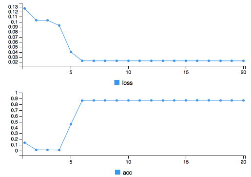
Training takes about 1 minute, and as can be seen from the training plot, it seems that both the loss and the accuracy have saturated. An accuracy of 0.9 sounds good, but let’s take a look at the output image before we get too happy.
First, we need to recreate the original dataframe with the predicted pixel values. For every \((x,y)\) pair in our matrix X we need to make a prediction. We duplicate the original dataframe fill the color channel columns with the network’s output values. We then call gather on this dataframe to create the cc and value columns necessary for the imager library.

df_out <- df
df_out[, 3:5] <- model %>% predict(X)
df_out <- df_out %>%
  gather(key = "cc", value = "value", -x, -y, convert = TRUE)

With the data frame in the right form, we can display the result next to the original image very easily. We convert the data frame to an image with the as.cimg function and paste it next to the original image by wrapping them inside a list and calling imappend on it, specifying we want them appended on the horizontal axis.

as.cimg(df_out) %>% list(im, .) %>%
  imappend("x") %>% plot(axes = F)

The network learned a gradient

The result is a vertical gradient, which can also be seen when looking at the model weights.

model$get_weights()

## [[1]]
##              [,1]         [,2]         [,3]
## [1,]  0.000755751  0.001207316  0.001467007
## [2,] -0.002216082 -0.004577803 -0.006758745
## 
## [[2]]
## [1] 1.460977 2.029516 2.619324

The values corresponding to the x column are positive, while the y values are negative and about one order of magnitute larger.

More layers

Now let’s try a network with more layers. More specifically, let’s add two layers with both 10 nodes followed by sigmoid activations.

model <- keras_model_sequential()
model %>%
  layer_dense(10, input_shape = 2, activation = "sigmoid") %>%
  layer_dense(10, activation = "sigmoid") %>%
  layer_dense(3, activation = "sigmoid")

model %>% compile(
  loss = "mean_squared_error",
  optimizer = optimizer_adam(),
  metrics = "accuracy"
)

model %>% fit(
  X, Y,
  batch_size = 128,
  epochs = 20
)

df_out <- df
df_out[, 3:5] <- model %>% predict(X)
df_out <- df_out %>%
  gather(key = "cc", value = "value", -x, -y, convert = TRUE)

as.cimg(df_out) %>% list(im, .) %>%
  imappend("x") %>% plot(axes = F)

Some features of the bird appear

As can be seen, the image is already picking up some countours of the bird, together with some ‘rays’ coming from the top-left corner. If we go for an even deeper network, more of the bird’s features can be recognized from the image.

model <- keras_model_sequential()
model %>%
  layer_dense(100, input_shape = 2, activation = "tanh") %>%
  layer_dense(100, activation = "relu") %>%
  layer_dense(100, activation = "relu") %>%
  layer_dense(100, activation = "relu") %>%
  layer_dense(100, activation = "relu") %>%
  layer_dense(3) %>% 
  layer_activation_relu(max_value=1)

model %>% compile(
  loss = "mean_squared_error",
  optimizer = optimizer_adam(),
  metrics = "accuracy"
)

model %>% fit(
  X, Y,
  batch_size = 128,
  epochs = 100
)

df_out <- df
df_out[, 3:5] <- model %>% predict(X)
df_out <- df_out %>%
  gather(key = "cc", value = "value", -x, -y, convert = TRUE)

as.cimg(df_out) %>% list(im, .) %>%
  imappend("x") %>% plot(axes=F)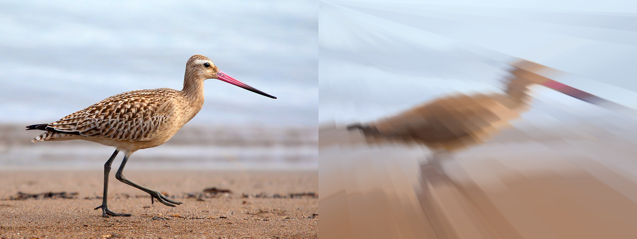

The image is nicely recovered

Ways to improve this might include more layers, more epochs, different activation functions, different loss function. For now, I’m really happy with the result!